Benchmarking Your Code to Justify a Resource Allocation Request
When you submit a Resource Allocation Request you are asking CRCD for a number of Service Units (SUs) — roughly, core-hours of computing time. A strong request answers one question with evidence rather than a guess:
How many SUs will my project actually consume, and how did you arrive at that number?
The most convincing way to answer is to benchmark a small, representative piece of your
workflow on the cluster, measure what it consumed, and extrapolate to the full project. This
page walks through that process end to end using the Amber molecular-dynamics job from
Requesting Resources as the running
example, and shows how to capture the numbers automatically with crc-job-stats.
About the numbers on this page
Every benchmark on this page uses real measurements from actual Amber jobs on the
mocvnhlysm system: the GPU example (Steps 1–7), the HTC CPU comparison, and the full MPI
strong-scaling study from 1 to 256 cores. Only the project scale (10 systems × 500 ns) is an
example — replace it with your own project plan.
Why benchmarking matters for an allocation
A Service Unit charge is not simply "one hour = one SU." On a running job Slurm computes a billing rate from the maximum of the weighted resources you requested — cores, memory, or GPU cards — and multiplies that rate by the job's walltime:
total SUs ≈ max(cores × compute_weight, GB × memory_weight, GPUs × compute_weight) × hours
The per-partition billing weights are listed on the Service Units page.
The ones used in this example (the GPU cluster's l40s partition) are:
| Cluster | Partition | Compute weight (per CPU/GPU) | Memory weight (per GB) |
|---|---|---|---|
| GPU | l40s |
8 | 0 |
Because the weights differ by partition and the charge is driven by whichever resource dominates, you cannot reliably estimate a project's cost from intuition. Benchmarking gives you a measured SU-per-unit-of-work figure that you can defend line by line in your request.
The workflow at a glance
- Instrument your Slurm script by adding
crc-job-statsas the last line. - Design a small benchmark that represents one well-defined unit of your real work.
- Run the benchmark (and, ideally, a short scaling study across resource choices).
- Read the
crc-job-statssummary to capture walltime and the allocated resources. - Convert the measured performance into Service Units using the billing weights.
- Extrapolate from one unit of work to the full project.
- Present the result as a short table in your allocation request.
Step 1 — Add crc-job-stats to your Slurm script
crc-job-stats is a CRCD wrapper meant to be placed at the very end of a Slurm submission
script. When the job reaches that line, it reads the job's metadata with scontrol and prints a
formatted summary — job ID, submit/end times, elapsed run time, the allocated trackable resources
(AllocTRES), the partition, the node list, and the command that ran — straight into your Slurm
output file. That output file becomes your benchmarking record.
Below is the exact Amber GPU script used to produce the real output on this page. The only
addition to a standard job is the last line, crc-job-stats.
#!/usr/bin/env bash

## ------------------------------------------------------------------
## Slurm directives defining the resource request
## ------------------------------------------------------------------
#SBATCH --job-name=gpus-1
#SBATCH --output=gpus-1.out
#SBATCH --nodes=1
#SBATCH --ntasks-per-node=1
#SBATCH --cluster=gpu
#SBATCH --partition=l40s
#SBATCH --gres=gpu:1
#SBATCH --time=24:00:00

## ---------------------------------------------------------------------
## Load software into environment
## ---------------------------------------------------------------------
module purge
module load amber/24-20260305

## ---------------------------------------------------------------------
## Setup software execution environment
## ---------------------------------------------------------------------
# Define environmental variables for Amber input/output files
INP=md.in
TOP=mocvnhlysm.top
CRD=mocvnhlysm.crd
OUT=mocvnhlysm

# Define software executable
SANDER=pmemd.cuda

# Display environmental variables to Slurm output file for diagnostics
echo AMBERHOME    $AMBERHOME
echo SLURM_NTASKS $SLURM_NTASKS
echo which SANDER `which $SANDER`
echo "Running on node:" `hostname`

# Display NVIDIA GPU information to Slurm output file
nvidia-smi

# Software execution line
$SANDER  -O     -i   $INP   -p   $TOP   -c   $CRD   -r   $OUT.rst \
                -o   $OUT.out   -e   $OUT.ene   -v   $OUT.vel   -inf $OUT.nfo   -x   $OUT.mdcrd

## ---------------------------------------------------------------------
## Report job statistics for benchmarking (add this line)
## ---------------------------------------------------------------------
crc-job-stats
Organize scaling studies by directory
The real job on this page was submitted from
.../benchmarking/gpu/mocvnhlysm_GPU_L40S-1C/. Encoding the system, cluster, GPU type, and
card count in the directory name (here, L40S with 1 card) keeps a scaling study tidy: one
directory per configuration, each with its own amber.slurm and gpus-1.out. The Command
field in the statistics block then records exactly which configuration produced which numbers.
Step 2 — Design the benchmark
A good benchmark measures a unit of work you can multiply. Decide up front:
- The unit. For MD, "1 ns of simulation" is a natural unit. For a training job it might be "one epoch"; for a parameter sweep, "one parameter set."
- How many units the full project needs. For example, 10 protein systems × 500 ns each.
- What you are varying, if anything. If you are unsure which resource to request, run the same unit of work under a few configurations — a scaling study — so you can justify the most efficient choice rather than the most expensive one.
Run enough steps for the throughput to stabilize
What matters is not wall-clock length but that the reported ns/day has reached steady
state. Amber averages performance over many steps, so even a short run can give a solid
number: the example on this page ran 50,000 steps (0.1 ns) in about 30 seconds, and its
ns/day for the last 49,500 steps and for all steps agree to within 0.04 % — a sign the
measurement is stable. Just make sure the run is past any warm-up so setup time does not
dominate the average.
For the Amber GPU job, a small scaling study might compare one L40S GPU against an A100, or
confirm that a single GPU is the right choice because pmemd.cuda does not speed up with more
cards for this system size. Submit each configuration as its own job (change only the #SBATCH
directives), each ending in crc-job-stats.
Step 3 — Run the benchmark
Submit the instrumented script as usual:
[user@login1 ~]$ sbatch amber.slurm
Submitted batch job 3817289
When the job completes, its Slurm output file (gpus-1.out in this example) contains everything
your normal run prints plus the statistics block appended by crc-job-stats.
Step 4 — Read the crc-job-stats output
This is the actual tail of gpus-1.out from the example job. The nvidia-smi banner at the top
confirms the hardware (one NVIDIA L40S, 46 GB), and the statistics block below is what
crc-job-stats printed:
Running on node: gpu-n69.crc.pitt.edu
...
|   0  NVIDIA L40S                    On  |   00000000:E1:00.0 Off |                    0 |
| N/A   34C    P8             34W /  350W |       0MiB /  46068MiB |      0%      Default |
...
==============================================================================
                                JOB STATISTICS
==============================================================================

           JobId: 3817289
      SubmitTime: 2026-09-08T08:42:04
         EndTime: 2026-09-09T08:42:05
         RunTime: 00:00:35
       AllocTRES: cpu=16,mem=125G,node=1,billing=8,gres/gpu=1
       Partition: l40s
        NodeList: gpu-n69
         Command: /vast/crcd/kimwong/benchmarking/gpu/mocvnhlysm_GPU_L40S-1C/amber.slurm

==============================================================================
 For more information use the command:
   - `sacct -M gpu -j 3817289 -S 2026-09-08T08:42:04 -E 2026-09-09T08:42:05`

 To control the output of the above command:
   - Add `--format=<field1,field2,etc>` with fields of interest
   - See the list of all possible fields by running: `sacct --helpformat`
==============================================================================
Three fields drive the costing, and one is a trap:
RunTime=00:00:35— the elapsed walltime, 35 seconds. Use this field for walltime.AllocTRES=cpu=16,mem=125G,node=1,billing=8,gres/gpu=1— the resources Slurm charged for. Note thebilling=8term: that is the job's per-hour SU rate.EndTime(the trap).EndTimeminusSubmitTimehere is about 24 hours, not 35 seconds. That is becausecrc-job-statsruns while the job is still active, soscontrolreportsEndTimeas your requested time limit (--time=24:00:00), not the real finish. Always take the walltime fromRunTime, never fromEndTime − SubmitTime.
Why billing=8 even though 16 cores and 125 GB were allocated
Requesting one GPU auto-allocated a proportional share of the node — 16 cores and 125 GB — but
on the l40s partition the memory weight is 0 and the rate is driven by the single GPU
(1 × 8 = 8). The 16 cores and 125 GB add nothing to the bill. This is exactly why measuring
beats guessing: the cost tracks the GPU, not the incidental CPU and memory.
crc-job-stats also prints the exact sacct command for a deeper look. Running it with a
--format that includes MaxRSS lets you record peak memory — useful on the CPU clusters, where
memory is weighted, though not needed here since GPU memory is free.
Step 5 — Convert the benchmark into Service Units
Cost of the run itself. Apply the billing=8 rate to the measured RunTime:
SUs for this run = 8 SU/hour × (35 s ÷ 3600 s/hour) ≈ 0.078 SUs
That confirms the rate, but a single 35-second run is not yet a unit you can multiply — it simulated only 0.1 ns (50,000 steps × 0.002 ps). For MD you want cost per nanosecond, which combines the billing rate with Amber's own throughput.
RunTime (35 s) vs Amber's wall time (31 s)
Amber reports Total wall time: 31 seconds for the compute kernel, while crc-job-stats
reports RunTime 00:00:35 for the whole job. The extra few seconds are module load,
nvidia-smi, and crc-job-stats itself. Slurm charges on the full job elapsed time, so
always cost from RunTime, not from the application's internal timer.
Cost per ns (Amber-specific). Amber prints its performance as ns/day in the "Final
Performance Info" block at the bottom of mocvnhlysm.out. This run reported 298.16 ns/day on
one L40S. Combine that with the billing=8 rate:
SU per ns  =  billing rate (SU/hour) × 24 (hour/day)  ÷  throughput (ns/day)
           =  8 × 24 ÷ 298.16
           =  192 ÷ 298.16
           ≈  0.64 SUs per ns
Cost per unit (general method). For codes that do not report throughput, run the benchmark
long enough to complete exactly one unit of work and read RunTime directly:
SU per unit = billing rate (SU/hour) × RunTime (hours)
Let the tools confirm finished jobs
For the exact charge on a completed job you can also use crc-seff, or the sacct command
crc-job-stats prints. Use the hand formula above for extrapolating to work you have not
run yet.
Step 6 — Extrapolate to the full project
Multiply the measured per-ns cost by the total nanoseconds your project requires. Suppose the project is 10 systems simulated to 500 ns each, at the measured 0.64 SU/ns from Step 5:
Total ns          =  10 systems × 500 ns    =  5,000 ns
Total SUs         =  5,000 ns × 0.64 SU/ns  ≈  3,220 SUs
Add ~15% headroom for restarts, failed jobs, and analysis:
Requested SUs     ≈  3,700 SUs
As a cross-check, 5,000 ns at 298.16 ns/day is about 16.8 days = 402 hours of walltime; at 8 SU/hour that is ≈ 3,220 SUs — the same subtotal, reached the other way.
Building in a modest safety margin is expected and reasonable — jobs occasionally fail, restart, or need re-running, and analysis steps consume SUs too. State the margin explicitly so reviewers see it is deliberate.
Step 7 — Present it in your allocation request
Turn the above into a compact, defensible table. This is the kind of justification reviewers can verify at a glance:
| Quantity | Value | Source |
|---|---|---|
| Benchmark system | mocvnhlysm, 50,000 steps (0.1 ns) on one NVIDIA L40S |
mocvnhlysm.out / nvidia-smi |
| Partition / resources | GPU cluster, l40s, 1 GPU (16 cores, 125 GB co-allocated) |
AllocTRES |
| Billing rate | 8 SU/h | AllocTRES billing=8 |
| Measured throughput | 298.16 ns/day | Amber mocvnhlysm.out |
| SUs per ns | ≈ 0.64 SU/ns | 192 ÷ 298.16 |
| Total ns required | 5,000 ns (10 systems × 500 ns) | project plan |
| Subtotal | ≈ 3,220 SUs | 5,000 × 0.64 |
| Headroom (~15%) | ≈ 480 SUs | restarts + analysis |
| Total requested | ≈ 3,700 SUs | — |
A short paragraph should accompany the table explaining the unit of work, the benchmark
configuration, and why the requested resources (here, a single l40s GPU rather than multiple
cards) are the efficient choice — ideally citing a small scaling study.
Worked examples across clusters
The seven-step method above is the same on every cluster — only the unit of work, the billing driver, and how you justify the resource count change. The tabs below give a starting job script for each cluster; the analysis that follows each is what belongs in your request.
#SBATCH --job-name=gpus-1
#SBATCH --output=gpus-1.out
#SBATCH --nodes=1
#SBATCH --ntasks-per-node=1
#SBATCH --cluster=gpu
#SBATCH --partition=l40s
#SBATCH --gres=gpu:1
#SBATCH --time=24:00:00

module purge
module load amber/24-20260305
# ... application setup and execution ...
crc-job-stats
#SBATCH --job-name=htc
#SBATCH --output=htc.out
#SBATCH --nodes=1
#SBATCH --ntasks-per-node=128
#SBATCH --cluster=htc
#SBATCH --partition=htc
#SBATCH --time=24:00:00

module purge
module load amber/24-20260305
# ... Amber input/output variables ...
SANDER=pmemd.MPI
mpirun -n $SLURM_NTASKS \
    $SANDER -O -i md.in -p mocvnhlysm.top -c mocvnhlysm.crd -r mocvnhlysm.rst \
               -o mocvnhlysm.out -e mocvnhlysm.ene -v mocvnhlysm.vel \
               -inf mocvnhlysm.nfo -x mocvnhlysm.mdcrd
crc-job-stats
#SBATCH --job-name=mpi
#SBATCH --output=mpi.out
#SBATCH --cluster=mpi
#SBATCH --partition=ndr
#SBATCH --nodes=2               # ndr enforces a minimum node count
#SBATCH --ntasks-per-node=128   # 2 x 128 = 256 ranks
#SBATCH --time=2:00:00

module purge
module load amber/24-20260305
SANDER=pmemd.MPI
mpirun -n $SLURM_NTASKS \
    $SANDER -O -i md.in -p mocvnhlysm.top -c mocvnhlysm.crd -r mocvnhlysm.rst \
               -o mocvnhlysm.out -e mocvnhlysm.ene -v mocvnhlysm.vel \
               -inf mocvnhlysm.nfo -x mocvnhlysm.mdcrd
crc-job-stats
Benchmarking sub-node core counts fairly
ndr enforces a minimum node allocation, so the 1–128-core points were run on a single
HTC node with #SBATCH --constraint=amd,turin to pin the same AMD Turin processor used
in ndr. That keeps per-core performance comparable across the whole 1→256 sweep; only the
128→256 step crosses from one node to two.
GPU — the GPU sets the price
This is the fully worked example in Steps 1–7. On l40s the billing rate is driven by the
single GPU (billing=8), memory is free (weight 0), and the co-allocated CPU cores do not add to
the cost. The justification is simply SU/ns × total ns, plus a note (ideally a one-GPU vs
multi-GPU comparison) that one card is the efficient choice for this system size.
HTC — same job, and why benchmarking changed the decision
The HTC cluster caps jobs at a single node, but that node is large — this run used the CPU build
pmemd.MPI across 128 cores to simulate the same mocvnhlysm system as the GPU example.
Because it is the identical workload and the same 50,000-step (0.1 ns) run as the GPU benchmark,
it is a direct, honest CPU-vs-GPU cost comparison (the MPI scaling study below uses separate,
shorter 1,000-step runs). Its
crc-job-stats block reported:
           JobId: 11178723
         RunTime: 00:19:27
       AllocTRES: cpu=128,mem=1000G,node=1,billing=128
       Partition: htc
        NodeList: htc-n77
On htc the weights are 1 SU/core-hour and 0.128 SU/GB-hour, so both terms happen to tie here
(128 cores × 1 = 128, 1000 GB × 0.128 = 128) and the rate is billing=128 — sixteen
times the GPU job's rate of 8.
Choose the steady-state throughput, not the all-steps average
Amber's mocvnhlysm.out reported two very different figures: 7.44 ns/day averaged over
all steps but 31.55 ns/day over the last 4,000 steps. The gap is a large one-time
startup cost (MPI init, filesystem warm-up) that does not recur proportionally in long
production runs, so the steady-state figure (31.55 ns/day) is the fair basis for extrapolation
— provided your production jobs run long enough to amortize that startup. This run's short
0.1 ns length is exactly why the two disagree; a longer benchmark would narrow the gap. On the
GPU the two figures were within 0.04 % of each other, so this only bites on the slower CPU run.
Costing it out at the favorable steady-state rate:
SU per ns (HTC, steady state) = 128 × 24 ÷ 31.55 ≈ 97 SUs per ns
Set that beside the GPU result of 0.64 SU/ns and the benchmark makes the decision for you:
| Cluster | Rate | Throughput | SU per ns | 5,000-ns project |
|---|---|---|---|---|
GPU l40s, 1 GPU |
8 SU/h | 298 ns/day | 0.64 | ≈ 3,200 SUs |
HTC htc, 128 cores |
128 SU/h | 31.6 ns/day (steady) | 97 | ≈ 487,000 SUs |
For this workload the GPU is roughly 150× cheaper per nanosecond (and ~640× if you use the all-steps CPU figure). That is the single most persuasive thing a benchmark can show a reviewer: not just how many SUs you need, but that you measured the alternatives and chose the efficient one. The lesson is workload-specific — a code with no GPU port, or one that is memory-bound, may favor HTC — which is precisely why you benchmark rather than assume.
The CUDA warning in htc.out is harmless
The CPU run prints CUDA-aware support is disabled ... libcuda.so.1: cannot open shared object
file. That is OpenMPI noting there is no GPU on the HTC node; it does not affect a CPU-only
pmemd.MPI run and can be ignored (or silenced with --mca opal_warn_on_missing_libcuda 0).
MPI — justify the core count with a scaling study
For a multi-node MPI code the central question a reviewer asks is why this many cores? Answer it
with a strong-scaling study: run the same fixed problem (here nstlim=1000, unchanged
across every job) at 1, 2, 4, … cores, take each throughput from Amber's ns/day — cross-checked
against the crc-job-stats RunTime — and plot speedup and the resulting SU cost.
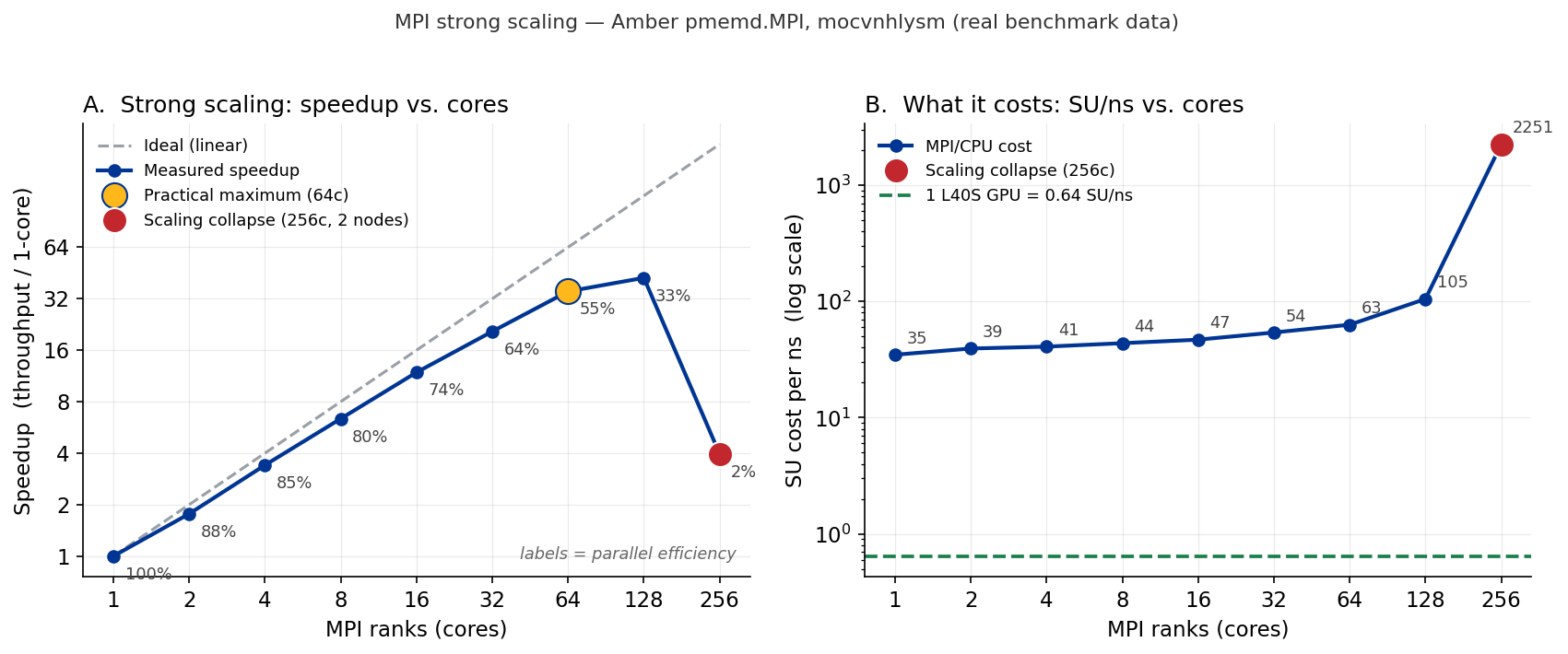
Read the figure the way a reviewer will. On both htc and ndr the billing weight is 1 SU per
core-hour, so a job's rate equals its core count (confirmed by the billing= field in every
crc-job-stats block). Under perfect scaling, cost per ns would be constant; real codes fall
off the ideal line, and the moment they do, more cores buy less speed per SU:
| Cores | Throughput (ns/day) | Speedup | Parallel efficiency | SU per ns | vs. GPU |
|---|---|---|---|---|---|
| 1 | 0.69 | 1.00× | 100% | 35 | 54× |
| 2 | 1.22 | 1.77× | 88% | 39 | 61× |
| 4 | 2.35 | 3.41× | 85% | 41 | 63× |
| 8 | 4.39 | 6.36× | 80% | 44 | 68× |
| 16 | 8.19 | 11.87× | 74% | 47 | 73× |
| 32 | 14.21 | 20.59× | 64% | 54 | 84× |
| 64 | 24.36 | 35.30× | 55% | 63 | 98× |
| 128 | 29.24 | 42.38× | 33% | 105 | 163× |
| 256 | 2.73 | 3.96× | 2% | 2,251 | 3,495× |
Throughput is Amber's all-steps ns/day, chosen because it is well-defined at every core count —
at 1–2 cores Amber's "last-N steps" window collapses to a single step and is unreliable — and
because it tracks the crc-job-stats RunTime: across all nine jobs the reported RunTime
exceeds Amber's internal wall time by only 0–3 seconds (module load, mpirun launch, and
crc-job-stats itself). Note this is also why the raw RunTime is not the scaling metric: on
these sub-10-second runs the fixed launch overhead is visible (128 cores took 11 s of RunTime
versus 9 s at 64 cores, even though its compute was faster), so throughput, not wall-clock,
is what scales cleanly.
Two findings drive the request. First, scaling is healthy through 64 cores (35× speedup, still 55% efficient); at 128 cores efficiency has fallen to 33%, and going to 256 cores — the first configuration that spans two nodes — collapses throughput back to roughly the 4-core level (a 3.96× speedup versus 3.41× on just 4 cores) while costing 2,251 SU/ns. Inter-node communication overwhelms this small system, a textbook strong-scaling limit. So the defensible MPI request is single-node, in the 16–64-core range: cite the efficiency at your chosen count and note explicitly that you tested up to 256 cores and ruled it out.
Benchmarking revealed the efficient platform
Even the cheapest MPI point (1 core, 35 SU/ns) is ~54× the GPU's 0.64 SU/ns, and the fastest MPI configuration (128 cores, 29 ns/day) reaches only ~10% of a single L40S's 298 ns/day. For this Amber workload the benchmark is unambiguous: request the GPU. The scaling study still earns its place in the proposal — it is the evidence that CPU/MPI was evaluated and rejected, and it is exactly the analysis you would rely on for a code with no GPU port.
Side-by-side summary
| Cluster | Benchmark unit | Billing driver (weights) | What justifies the request |
|---|---|---|---|
GPU (l40s) |
0.1 ns of MD | GPU card (8/GPU, 0/GB) | 0.64 SU/ns — ~50–3,500× cheaper than any CPU config |
HTC (htc) |
0.1 ns of MD, single node | cores (1/core) or memory (0.128/GB) | ~97 SU/ns on 128 cores; direct CPU-vs-GPU comparison |
MPI (mpi/ndr) |
fixed 1,000-step run | cores (1/core, 0.093/GB) | scaling study: efficient to ~64 cores, collapses at 256 |
Tips and common pitfalls
- Take walltime from
RunTime, notEndTime − SubmitTime. While a job is running,scontrolreportsEndTimeas the requested time limit, so the difference overstates the real elapsed time — sometimes by hours, as in the 35-second example above. - Benchmark on the cluster and partition you will request. Billing weights and hardware differ between clusters, so a timing from your laptop or a different partition will not convert correctly.
- Match the real work. Same system size, same settings, same code path — only the number of steps should be smaller. A benchmark that skips the expensive part will underestimate the request.
- On the GPU cluster, memory is free. The
l40smemory weight is 0, so the 125 GB co-allocated with your GPU adds nothing to the bill; the GPU count sets the rate. On the CPU clusters memory is weighted, so there record peak usage (MaxRSSviasacct, orcrc-seff). - Test at zero cost first. You can shake out a script on a
preemptpartition, where billing weights are 0, before running the timed benchmark that will inform your numbers. See Preemptible Partitions. - Check your standing.
crc-usageshows how many SUs your group has used and has remaining, which helps you frame the size of the new request.
Reference: commands used on this page
| Command | Purpose |
|---|---|
crc-job-stats |
Append a job-statistics summary (RunTime, AllocTRES, partition, nodes) to the Slurm output file. Place it as the last line of your script. |
crc-seff |
Report the efficiency and billed resources of a completed job. |
crc-usage |
Show your group's SU usage and remaining balance. |
sacct -M <cluster> -j <JobID> --format=User,JobID,JobName,AllocTRES%40,Elapsed |
Inspect the billing components (AllocTRES) and elapsed time of a job. |
scontrol -M <cluster> show partition |
Read a partition's TRESBillingWeights directly. |
Related pages
- Requesting Resources — anatomy of the Slurm script used above.
- Service Units — the billing model and full weight table.
- Job Limits & QoS — per-group caps that are separate from cost.
- Resource Descriptions for Writing Proposals — describing CRCD hardware in a grant or allocation proposal.
- Resource Allocation Request form — where the justification goes.